Normal distribution
A useful continuous distribution is the normal distribution with mean equal to
0 and standard deviation equal to 1. It can be shown that
the
area under the standard (i.e., mean=0, standard deviation=1) normal
distribution from negative
infinity to infinity is equal to 1. In
order to find the relative frequency of being in an interval (which we shall
later call the probability of being in an interval), the area under the
normal curve to the left of a cutoff has been tabulated. You will need to use
a table, but with a table you will be able to answer the following questions:
Tables have tabulated the area under the standard normal curve to the
left of a specified z-value (the letter z generally refers to standard normal
distribution (mean=0, variance=1); caveat: some tables record the
area between 0 and the specified cutoff). We can find the area (or relative
frequency or probability) associated with an interval by calculating the
difference of the areas associated with the endpoints. Thus to find the area
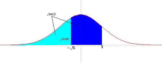
over the interval (-.5, 1) which is shaded in blue in the figure below,

we find in a table of the normal distribution associated with the z-value 1
the area .8413 (which corresponds to the blue and cyan regions in the figure),
and we find in the table associated with the z-value -.5 the area .3085 (which
corresponds to the cyan area in the figure). Subtracting provides that the
area
of the blue region is .8413-.3085=.5328. Recall that the total area under the
curve is 1, hence the area to the right of a cutoff can be found by subtracting
the area to the left of the cutoff from 1. The area to the right of 1 (white
in the figure) is 1-.8413=.1587. N.B.: All areas (relative frequencies,
probabilities) will be between 0 and 1, inclusive.
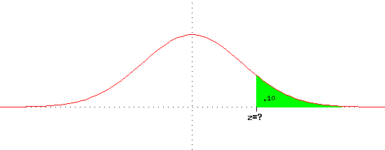
If we wanted to know what z-value 10% of the data would be above (or the
data would be above 10% of the time), we would want the the area under the
curve beyond the z-value to be equal to .10 (the green shaded region in the
figure below).

That means that the area under the curve to the left of the z-value (white in
the figure) would be .9. Looking for .9 in the body of the table, we find
.8997 and .9015, which correspond to the z-values 1.28 and 1.29, respectively.
Thus the area to the right of z=1.28 is .1 (actually .1003).
DO NOT BE AFRAID TO DRAW A PICTURE WHEN DOING PROBLEMS OF THIS NATURE. It is
important to distinguish between z-values (which may be any real number) and
the corresponding areas (probabilities, relative frequencies) which are between
zero and one, inclusive).
ALSO, remember that with continuous distributions, it does not matter whether
inequalities are strict or weak (the probability of a specific value is 0).
Competencies: If X is normally distributed with mean 0 and standard
deviation 1 (N(0,1)), what is the probability that .5 < X < 2 ?
If X is normally distributed with mean 0 and standard deviation 1 (N(0,1)),
what value will X be less than 30% of the time?
return to index
Questions?

